Recall that loops carrying no dependences can be parallelized or vectorized. The recursive version of the vectorize algorithm made use of this by descending down the levels in a loop-nest and satisfying loop-carried dependences that created loops in dependence graphs by serializing loops until all dependence cycles were broken and the remaining loops could be vectorized. However, simply applying the vectorize algorithm (or an equivalent algorithm to parallelize outer loops) on raw source codes misses several opportunities. Consider the following example.
  for i = 1:N {
    for j = 1:M {
S     A(i,j+1) = A(i,j) + B;
    }
  }
The above loop-nest has a dependence from the statement S to itself that is carried by the j-loop. The recursive vectorize algorithm will fail to vectorize the nest, even though a simple transformation can make the loop-nest partially vectorizable. Suppose we interchanged the i- and the j-loops. Notice that the dependence vector is (=,<), which becomes (<,=) after interchanging the loops. It should be obvious that the new direction vector can be obtained by simply reordering the entries in the vector, corresponding to the interchanges of the loops. Here, the two loops are swapped and so are the corresponding direction-vector entries. Notice that the interchange is legal because the source and the sink of the dependence are still executed in the same order as before, thus preserving the dependence. With the loop-interchange, the inner loop becomes free of dependence cycles and can be vectorized by the recursive vectorize algorithm.
In general, to fruitfully parallelize or vectorize loops the loops must be transformed to expose parallelism that may not be available in the original form. These notes discuss a few of such loop transformations.
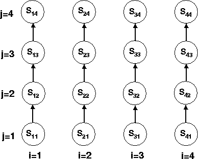
One way to understand the legality of this loop interchange is to visualize the iteration space. Suppose that we use Cartesian coordinates to represent the two-dimensional iteration vector space as shown in the figure below. The statement S in the above loop-nest has a dynamic instance corresponding to each point in the iteration space. It is easy to verify that the arrows in the figure are the dependences in the above loop. For each arrow, the statement instance at its source writes the memory location that is read by the statement instance at the sink of the arrow.

In the original loop nest, i-loop is the outer loop, meaning that all the statement-instances in the left column are executed (bottom-to-top) before those in the next column get executed. Loop interchange changes the order of execution of the statement-instances such that all the instances in the bottom row are executed (left-to-right) before the next row gets executed. Clearly, all the dependences are preserved since the sources of the dependence arrows are still executed before their corresponding sinks.
The effects of loop interchange on a dependence can be seen easily using the direction vector. Recall that a dependence to be valid the leftmost non-= entry in its directions vector must be “<”. Suppose that we apply a permutation, π, to a loop-nest. The direction vector for a dependence in the permuted loop-nest can be derived by applying the permutation π to the direction vector for that dependence in the original loop-nest. In order to see the effect of a loop-permutation on all the dependences in a loop-nest we define a direction matrix as follows:
A direction matrix is simply a row-wise listing of all distinct direction vectors in a loop-nest. Consider the following loop-nest:
   for i = 1:N {
     for j = 1:M {
       for k = 1:L {
S1       A(i+1,j,k) = B(i+1,j,k-1) + c;
S2       B(i+1,j+2,k-1) = A(i,j,k+1) + B(i,j+2,k) + D;
       }
     }
   }
There are three dependences in the above loop:
 <  =  >
 =  <  =
If we were to interchange the i-loop and the j-loop we would get the following direction matrix.
 =  <  >
 <  =  =
Since all the dependences are still valid this interchange is legal. However, interchanging the i-loop with k-loop is not legal since that causes the first row of the direction matrix to have a “>” in the leftmost non-= position, which indicates violation of a dependence. Direction matrices provide an easy mechanism to determine which loop-interchanges are legal without having to carry out any code transformation.
Loop-interchanges by themselves are not always enough to enable parallelism. Consider the following loop-nest.
for i = 1:N {
  for j = 1:M {
    A(i,j) = A(i-1,j) + A(i,j-1);
  }
}
The statement has two carried dependences to itself with the following dependence matrix:
 =  <
 <  =
If we interchange the loops the new outer loop still carries one of the dependences. We can visualize these
dependences as before by drawing the dependences among statement-instances over the iteration space. No matter
in which order we go through the iterations—column-major or row-major—the carried dependences
prevent us from parallelizing the loop.
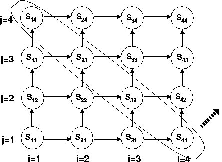
However, we can “skew” the loop-nest so that the inner-loop iterates over the statement-instances along a diagonal in the above picture. So, the circled statement-instances get executed in one iteration of the outer loop and the outer loop proceeds in the direction of the dashed arrow. Now the inner loop can be vectorized. One way to think about loop-skewing is that we align the iteration space coordinates differently (at a 45° angle, in this case) and re-label the statement instances in the new coordinates.
Observe that the diagonal that we want to execute in the inner loop has the equation of the form i+j=c, where c is a constant 2, 3, 4, ... (N+M). Based on this observation we can rewrite the inner loop in terms of c, instead of j. We note the following relations:
c = i + j
j = c - i
Thus, as j goes from 1 to M, c goes from i+1 to i+M.
Substituting the values of j in the subscripts in terms of c, we get the following skewed
loop-nest.
for i = 1:N {
  for c = i+1:i+M {
    A(i, c-i) = A(i-1, c-i) + A(i, c-i-1);
  }
}
If we compute the new direction matrix using the Delta method we get the following:
 =  <
 <  <
This does not seem to have accomplished anything, since dependences are still carried by both the loops. However, now, the loop can be interchanged so that serializing the outer loop in the interchanged loop-nest will satisfy all the carried dependences, leaving the inner loop free to be parallelized. However, we need to be careful about the loop-bounds since the new loop-nest is no longer “rectangular”.
for c = 2:N+M {
  for i = max(1,c-M), min(N,c-1) {
    A(i, c-i) = A(i-1, c-i) + A(i, c-i-1);
  }
}
The inner i-loop can now be parallelized.
Sometimes a loop-carried dependence can be eliminated by unfolding the first few iterations of a loop. This is called loop peeling, illustrated by the following example:
for i = 1:N {                     A(1) = A(1) + A(1)
  A(i) = A(i) + A(1);    =>       for i = 2:N {
}                                   A(i) = A(i) + A(1)
                                  }
The loop on the right hand side has no loop-carried dependences and can be parallelized.
Consider the following loop-nest.
   for i = 1:100 {
     for j = 1:100 {
S1       A(i,j) = B(i,j) + C(i.j);
S2       D(i,j) = A(i-1,j-1)*2.0;
     }
   }
There is a loop-carried dependence from S1 to S2 with the direction vector (<,<). Loop interchange does not help. Due to the forward flow of the dependence (i.e., in the direction of the program order) it is possible to execute all j-instances of S1 before any j-instance of S2. This is called loop-distribution. The loop-nest now becomes:
   for i = 1:100 {
     for j = 1:100 {
S1       A(i,j) = B(i,j) + C(i.j);
     }
     for j = 1:100 {
S2       D(i,j) = A(i-1,j-1)*2.0;
     }
   }
Now the two j-loops can be individually vectorized. Notice that there is still a dependence between S1 and S2, now carried by the i-loop with the direction vector (<). Why does the direction vector have only one element? Once again, we can argue the same way we did before and distribute the i-loop, resulting in the following two separated loop-nests that can be completely parallelized.
   for i = 1:100 {
     for j = 1:100 {
S1       A(i,j) = B(i,j) + C(i.j);
     }
   }
   for i = 1:100 {
     for j = 1:100 {
S2       D(i,j) = A(i-1,j-1)*2.0;
     }
   }
In this particular case if statements S1 and S2 had been in the reverse order in the original code we could not have directly distributed the loops, however if we reordered the statements without violating any dependences then distribution would still apply. Which graph-based technique can be used here (that we have seen before) that can help us with reordering the statements to enable loop-distribution?
Another use of loop-distribution is in isolating parts of the loop that can be parallelized, as in the following simple loop:
   for i = 1:N  {
S1     A(i) = B(i) + 1;
S2     C(i) = A(i) + C(i-1);
S3     D(i) = A(i) + X;
   }
S2 has a loop-carried dependence on itself that prevents parallelization of the entire loop. On closer inspection we realize that no other statements are involved in any loop-carried dependences. So, distributing the loop around the three statements give us two parallelizable loops—the middle loop can still not be parallelized due to the loop-carried dependence.
   for i = 1:N  {
S1     A(i) = B(i) + 1;
   }
   for i = 1:N  {
S2     C(i) = A(i) + C(i-1);
   }
   for i = 1:N  {
S3     D(i) = A(i) + X;
   }
An alternative to loop distribution is possible in certain cases. Instead of executing all instances of the source of a dependence in a separate loop, the statement instances may be shifted across the iteration space to convert the loop-carried dependence into a loop-independent dependence. To accommodate the shifting the iteration space has to be usually expanded a little. The following example illustrates the transformation.
   for i = 2:N  {
S1     A(i) = B(i) + C(i);
S2     D(i) = A(i-1) * 2.0;
   }
The loop-carried dependence from S1 to S2 prevents parallelization. However, we could execute the instances of S2 one step ahead, giving rise to the following loop-nest:
   for i = 1:N+1  {
S1     if (i > 1) A(i) = B(i) + C(i);
S2     if (i ≤ N) D(i) = A(i-1) * 2.0;
   }
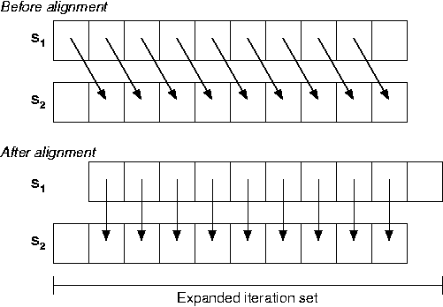
How can you get rid of the if conditions inside the loop? The idea behind loop-alignment is illustrated in the following figure.
The inverse of loop-distribution is loop-fusion. Loop-fusion is especially useful when loop-distribution has been applied and some of the resulting loop-nests may be fused together to increase the granularity of parallelism. Consider the last example that we saw when discussing loop-distribution. The distribution yields three loops, let's call these loops L1, L2, and L3. If we constructed a dependence graph between these loops by coalescing all the nodes in the original dependence graph that belonged to each loop into one single node representing the loop, we would get the following graph.
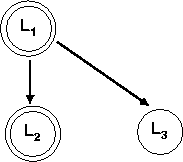
Since there is no dependence between L2 and L3 the two loops may be reordered. After the reordering, L1 and L3 can be fused again resulting in the following final code, which has a single parallel loop.
   for i = 1:N  {
S1     A(i) = B(i) + 1;
S3     D(i) = A(i) + X;
   }
   for i = 1:N  {
S2     C(i) = A(i) + C(i-1);
   }
Clearly, fusion may not always be possible. A simple modification to the above loop-nest,
   for i = 1:N  {
S1     A(i) = B(i) + 1;
S2     C(i) = A(i) + C(i-1);
S3     D(i) = A(i) + C(i);
   }
introduces a fusion-preventing edge in the dependence graph on the distributed loops,
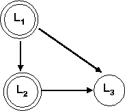
thus, preventing us from fusing L1 and L2. Loop fusion is a powerful technique to enhance the practicality of parallelism. An elaborate typed-fusion algorithm tries to produce maximally fused loops out of a given set of loops. A caveat is that sometimes fusing too many loops increases the register pressure in the compiler resulting in register spilling—meaning that too many values become live in the loop to be held in machine registers, giving rise to memory accesses where distributed loops may have none (or few). In practice, the cost of increased memory accesses must be balanced against the benefit of increased granularity of parallelism.
Sometimes, indiscriminate fusion may reduce parallelism! Consider the following code:
   for i = 1:N  {
S1     A(i+1) = B(i) + C;
   }
   for i = 1:N  {
S2     D(i) = A(i) + E;
   }
The two loops are parallelizable, and it is tempting to fuse the two together. However, fusion results in the following code,
   for i = 1:N  {
S1     A(i+1) = B(i) + C;
S2     D(i) = A(i) + E;
   }
which introduces a loop carried dependence from S1 to S2 preventing parallelization. Even though it is a powerful technique loop fusion must be applied carefully.
We have discussed a few of the loop-transformations, and there are several others that have been found to be useful from years of research. One question that comes up is: In which order should these loop-transformations be applied? In fact, we can generalize the question a bit and ask: At any stage of the code, how should we choose which loop-transformation to apply and when can we be sure that we can no longer improve the code?
Unfortunately, there is no simple answer to this question. Indeed, the question is closely linked to the open research problem in compilers of optimal ordering of program transformations. The problem is undecidable in the worst case and may be NP-hard in the best case. The challenge is to find an ordering that works for all applications. Strategies to solve this problem fall in three broad categories:
The problem of determining if a sequence of transformations really improves the performance of a piece of code is also open. In certain cases, such as when transformations uncover parallelism, the benefits are obvious. In other cases the benefits have to be weighed against potential costs, such as in the case of loop-fusion discussed earlier.
An aspect of dependence-based analysis that we have not discussed is handling of control-flow. For example, parallelizing a loop that has an if statement inside the loop body. There are two broad techniques to handle control-flow:
A loop-nest in which not all statements occur inside the innermost loop is called an imperfectly nested loop-nest. A loop in which either the upper or the lower bound, but not both, depend on a loop index of a surrounding loop, is a triangular loop. Which triangular loop-nest have we seen before? Was that loop-nest perfect? A loop in which both lower and upper bounds depend on the loop-indices of a surrounding loop, is a trapezoidal loop-nest. Have we come across a trapezoidal loop-nest in our discussions?
All of our discussion has focused on transforming perfect rectangular loop nests. It is possible to extend the dependence theory to a wider class of loops. Set-based representation (such as in Pugh's Omega Test paper) can be helpful in handling such cases.
B629, Arun Chauhan, Department of Computer Science, Indiana University